 is computed following equation (1).
Before the Iteration simulation of the TSG, the FRF simulation should be needed. Because, the Iteration simulation uses inverse FRF function.
The first drive signal is computed following equation (1).
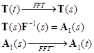 (1)
(1)
Where,  and
and  are the target signals on the time
domain and inverse FRF function, respectively.
are the target signals on the time
domain and inverse FRF function, respectively.
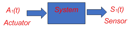
Figure 1 First simulation of the Iteration simulation
The first simulation with the first drive signals. Then
error signals ( ) of the first simulation can be
computed with following equation (2).
) of the first simulation can be
computed with following equation (2).
 (2)
(2)
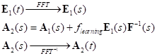
The drive signal  of the second simulation is computed
following equation (3).
of the second simulation is computed
following equation (3).
 (3)
(3)
Where,  is a scalar value and called a
learning factor. The learning factor cannot be 0.0.
is a scalar value and called a
learning factor. The learning factor cannot be 0.0.
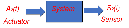
Figure 2 Second simulation of the Iteration simulation
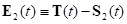
After second simulation, we can compute the second error
signals  again.
 (4)
(4)
In the case of the other simulation step, the second simulation procedure is repeated.
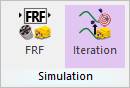
Figure 3 Iteration icon of the Simulation group in the TSG tab
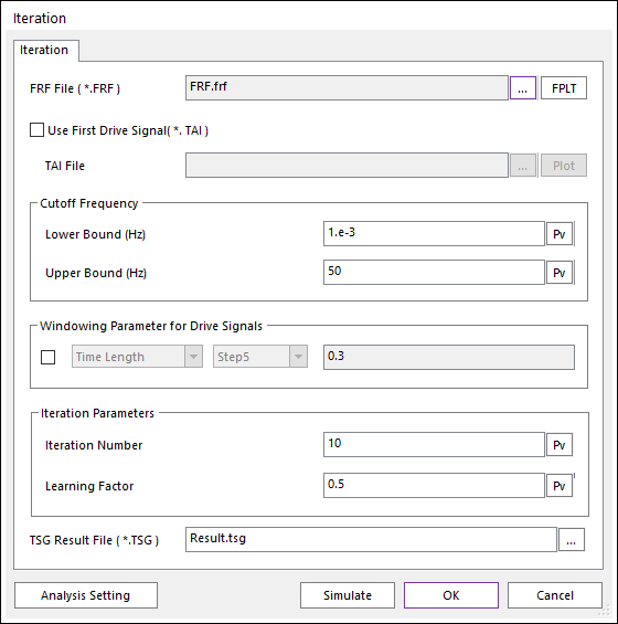
Figure 4 Iteration dialog box
•FRF File (*.FRF): Defines “*.FRF” file by clicking ….
•FPLT: Checks the FRF and the inverse FRF functions in the plot window.
•Use First Drive Signal (*.TAI): Default is unchecked. If this is checked, then the first drive signal is replaced the user selected signals in the input “*.TAI” file instead of equation (1).
•TAI File: If the Use First Drive Signal (*.TAI) is checked, then a “*.TAI” file should be set using “…” file. The “*.TAI” file can be generated Export function in FRF Result and Result dialogs.
•Plot: If a “*.TAI” file is selected, then User can see the signal data on the opened scope dialog.
•Cutoff Frequency: In order to ignore data of the inverse FRF this option is needed. Data of inverse FRF is between the Lower Bound and the Upper Bound frequencies is used to compute the next Drive Signal.
•Lower Bound (Hz): Default is 0.0 Hz.
•Upper Bound (Hz): Default is 1000000.0 Hz
•Windowing Parameter for Drive Signals: If the check box is selected, then a windowing function will be considered. Linear trapezoidal function is always computed.
•Data Size: A natural value greater than 0 should be set. And the Data Size should be lower than the number of signal data.
•Linear/Step5 : Two interpolation function types are available for windowing function.
•Time Length (s): A real number greater than 0.0 should be set.
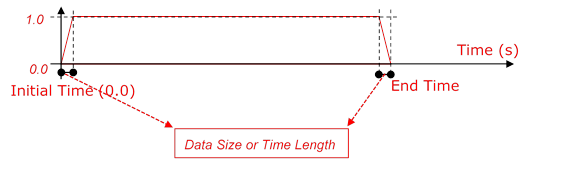
Figure 5 Windowing function for the Iteration simulation
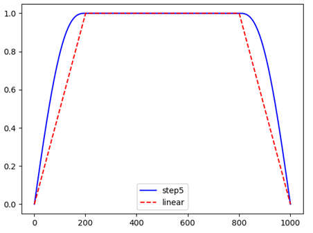
Figure 6 Comparison of the interpolation types for Windowing function
•Iteration Parameters
•Iteration Number: The simulation is repeated with the Iteration Number. Default is 1.
•Learning Factor: User can modify the learning factor  of equation (3). Default is
0.5. The range of the Learning Factor:
of equation (3). Default is
0.5. The range of the Learning Factor: 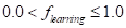 .
.
•TSG Result File (*.TSG): Defines the output “*.TSG” file saved all signal data.
•Analysis Setting: Dynamic/Kinematic Analysis dialog is opened. Because, currently TSG is only supported dynamic/kinematic analysis. The End Time and Step should be match on TSG setting.
•End Time data on the Dynamic/Kinematic Anlaysis dialog should be the same with the End Time of “*.TARGET” data.
•Step data on the Dynamic/Kinematic Anlaysis dialog should be set with (End_Time * Sampling_Frequency).
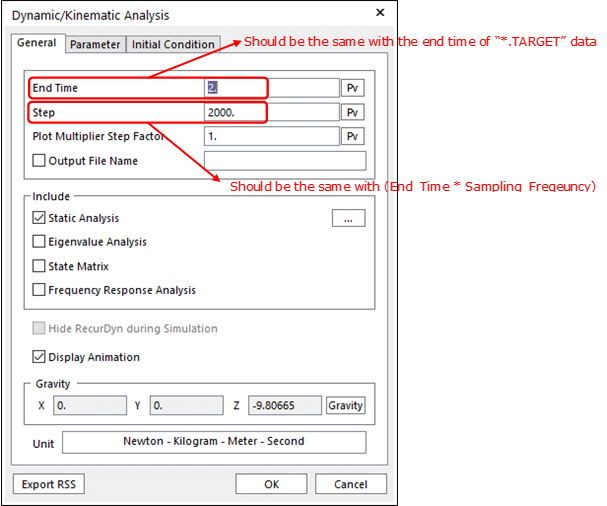
Figure 7 Dynamic/Kinematic Analysis dialog box
•Simulation: The Iteration simulation is started.
Usage the Iteration simulation of TSG
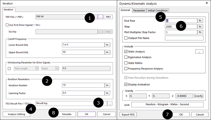
1. Set “*.FRF” file.
2. Set the Iteration Number.
3. Set the output “*.TSG” file name and path.
4. Click Analysis Setting.
5. Set the End Time on the Dynamic/Kinematic Analysis dialog. The End Time should be set the same value of the “*.TARGET” data.
6. Set the STEP on the Dynamic/Kinematic Analysis dialog. The Step should be the same with (End_Time * Sampling_Frequency).
7. Click OK on the Dynamic/Kinematic Analysis dialog to leave.
8. Click Simulate.