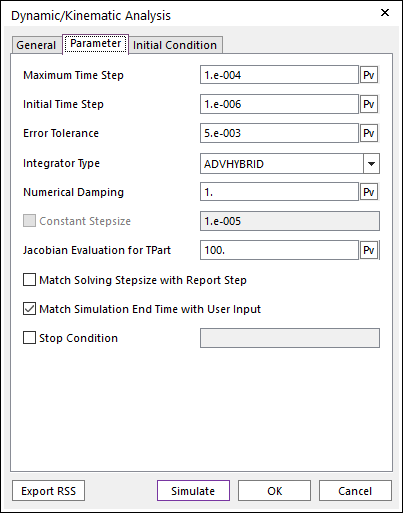
Figure 1 Dynamic/Kinematic Analysis dialog box [Parameter]
•Maximum Time Step: Defines the upper bound time step size of the integrator during the dynamic analysis. Since RecurDyn uses variable step size, the step size changes during simulation. Too small maximum time step can slower the simulation speed.
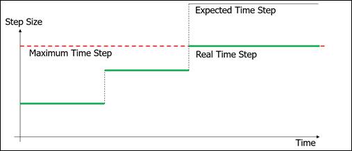
Figure 2 Maximum Time Step
•Initial Time Step: Defines the initial time step of the integrator during the simulation. In most of the cases, the default value 1.e-6 is good enough.
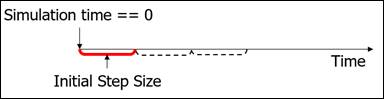
Figure 3 Initial Time Step
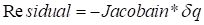
•Error Tolerance: Defines the error term used during the simulation
process. The system equations are solved using a Newton-Raphson method.
The Newton Raphson has converged when norm of  is less than a specified Error
Tolerance. Small error tolerance makes the simulation stricter. In most of
the cases, you can use the default value.
is less than a specified Error
Tolerance. Small error tolerance makes the simulation stricter. In most of
the cases, you can use the default value.
•
• : Vector of Generalized
Coordinates
: Vector of Generalized
Coordinates
•RecurDyn solves the equations of motion for general systems
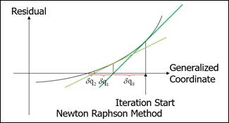
Figure 4 Newton Raphson Method
•Integrator Type: Allows selecting the integrator type. RecurDyn supports the Generalized-Alpha method [4].
•ADVHYBRID: Uses the Generalized-Alpha method.
o The system can contain any type of body.
o Appropriate for G-Modeling.
o The same integration method does not have to change when a body’s type is changed.
o Faster than other integrator methods for systems with RFlex bodies, especially when there are many modes or many connecting elements.
•IMGALPHA: Uses the Generalized-Alpha method.
o Systems with Rigid and/or RFlex bodies can be simulated.
o Tpart and FFlex bodies cannot be included.
•TRKGALPHA: Uses the Generalized-Alpha method.
o Systems with Rigid, RFlex, and/or Tpart bodies can be simulated. Tpart are special rigid bodies, which are Track HM/LM, Chain, Rigid 3D Belt.
o FFlex bodies cannot be included.
o Tpart bodies are Rigid bodies can only be connected using force elements.
o Tpart bodied cannot have constraints.
•HYBRID: Uses the Newmark method.
o Systems can contain any body types but must contain at least 1 FFlex body.
o Numerical damping has more effect than the other integrator types.
o The solution will be different than the other methods due to this numerical damping effect.
o When an FFlex body is added to a system that is originally simulated using the IMGALPHA or TRKGALPHA integrator, the integrator will automatically be switched to HYBRID.
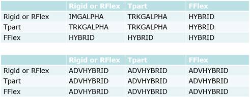
Figure 5 Integrator by Body types
•Numerical Damping: Defines the damping ratio for the generalized alpha method [4]. Parameters of Generalized-Alpha method are all a function of the numerical damping (ND). This can cause the damping effect even if there is no damper in the system. ND is required to be in the range 0<=ND<=1.
•ND = 0 implies no numerical damping, and ND = 1 implied maximum numerical damping.
•In real system, there are several kinds of damping effects which cannot be included in the model, so in most of the cases you can use the default value
•Constant Step Size: In the TRKGALPHA integrator, you can control the parameters of Constant Step Size. The Constant Step Size means the step size cannot change during simulation.
•Jacobian Evaluation for TPart: In the TRKGALPHA integrator, you can control the parameters of Jacobian evaluation. The Jacobian evaluation means the number of integration steps between each evaluation of Jacobian. For example, if the value is 100, the Jacobian system will be computed once per 100 integration steps. TPart are track links, chain links, and belt segments.
Note
The Jacobian Evaluation for TPart is a similar function to the Jacobian Evaluation Interval of the Advanced Solving Options on the Home tab.
If TRKGALPHA integrator is used, then the bigger parameter of the Jacobian Evaluation Interval and Jacobian Evaluation for TPart is only used. If the same value is set to both parameters, then Jacobian Evaluation Interval is only used.
•Match Solving Stepsize with Report Step: If you check this option, the solving step and report step are coincided. The step size of the animation is uniform (end time/steps). But the real step size of the solver or plot data is non uniform. So, you may not get the simulation result at the specific time instant. (for example, even if you want a result at 1.5s, the solver may calculate 1.47s then the next step can be 1.51 (step size is 0.04s). By checking this option, the solver calculates the time instants at N*end time/steps and match the animation step and the plot step.
Note
Following toolkits use always the “Match Solving Stepsize with Report Step” option.
1. TSG
2. SPI (Standard Particle Interface) - External & Embeded
3. Particleworks of Communicator
•Match Simulation End Time with User Input: If you check this option, the simulation is finished at the user-defined End Time. (The default is checked.)
•Stop Condition: If this option is checked, you can define an expression function. If the input expression becomes true, solver is stopped. Here, the value that evaluates to true is a value greater than zero.

Figure 6 Stop Condition
•For example, if Ex1 is inputted to Stop Condition after AZ (1, 2)>40D is made by Expression (Ex1), the value of Ex1 is as follows. For more information, refer to How to use Relational Operators, How to use Logical Operators.
•If the angular difference to the z axis of the first marker and the second marker is bigger than 40 degrees, the value of Ex1 is 1 and the solver is stopped.
•If the angular difference to the z axis of the first marker and the second marker is less than 40 degrees, the value of Ex1 is 0.