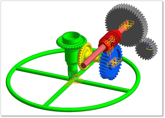
In the example model folder under the RecurDyn’s installation directory, open Gear_Model.rdyn. This model contains bevel gears, a helical gear and a worm gear. It was implemented using the GeoContact entity. The gear assembly is a dynamic model of a rotational machine system and requires the order tracking analysis. This model contains many possible joints and motions. This tutorial includes only those processes necessary to produce the Campbell diagram.
Example Model) <Install Dir>/Help/Examples/Campbell
Figure 1 Gear model
Creating the Expression
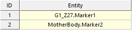
RevJoint2 of Subsystem1 contains the motion information and two reference markers: MotherBocy.Marker2 and G1_Z27.Marker1. The user will use these markers to produce an expression that can extract the necessary data.
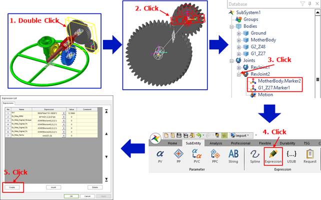
After performing the steps outlined in the preceding figure, the Expression List dialog box appears. This dialog box also includes the Expression dialog to create an expression. First, let's produce an expression that extracts the RPMs.
•Producing the RPM Expression
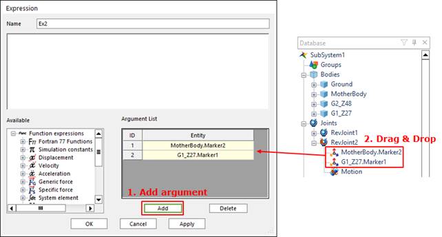
In the Name field for the expression, enter Ex_Mea_RPM. Then, drag two markers from the Database window and drop them in Argument List.
|
Expression |
60*WZ(1,2,2)/(2*pi) |
|
Argument List |
|
This expression multiplies the speed caused by the WZ function acting on the two markers by 60 and divides it by 2π to convert it into RPM. For more information about the WZ function, refer to the How to use Velocity Functions.
•Producing the Tacho Expression
Repeat the procedure for producing an RPM expression to create an expression that includes the two markers as arguments. Then, in the Name field for the expression, enter Ex_Mea_Tacho. Finally, enter the following information:
|
Expression |
sin(AZ(1,2)) |
|
Argument List |
|
This function enters the two markers into a sine function to produce the sine wave signal for each rotation. For more details on the AZ function, refer to the How to use Displacement Functions.
•Producing the Signal Fx Expression
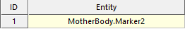
Create an expression named Ex_Mea_Signal_Fx. Then, drag MotherBody.Marker2 from the Database pane and drop it in the Argument List. Finally, enter the following information.
|
Expression |
JOINT(RevJoint2,0,2,1) |
|
Argument List |
|
This function extracts the reaction force of the joint by measuring the X-axis load of RevJoint2. In addition, the reference coordinate is MotherBody.Marker2. For more information about the Joint function, refer to the How to use Specific Force Functions.
•Producing the Signal Fy Expression
Create an expression named Ex_Mea_Signal_Fy. Input the same argument as for the Signal Fx expression, but enter JOINT(RevJoint2,0,3,1) for the expression. The user can also copy Ex_Mea_Signal_Fx, which was produced in the previous step, from the Database window and modify it.
|
Expression |
JOINT(RevJoint2,0,3,1) |
|
Argument List |
|
•Producing the Signal Fz Expression
Create an expression named Ex_Mea_Signal_Fz. Input the same argument as for the Signal Fx expression, but enter JOINT(RevJoint2,0,4,1) for the expression.
|
Expression |
JOINT(RevJoint2,0,4,1) |
|
Argument List |
|
•Producing the Torque for the Signal Fz Expression
Create an expression and named Ex_Mea_Signal_Torque. Input the same argument as for the Signal Fx expression, but enter JOINT(RevJoint2,0,8,1) for the expression.
|
Expression |
JOINT(RevJoint2,0,8,1) |
|
Argument List |
|
To produce the Campbell diagram, you need the following data: RPM or tacho data and signal data. For this tutorial, the user can input any load, acceleration, speed, and displacement data as the signal data. This sample extracts the RPM and tacho data as well as the reaction forces acting on the joint.
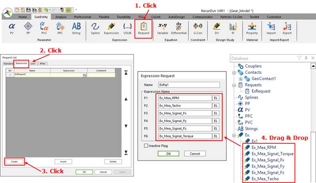
Creating the Request
To display the output of the expression, the user must register a request. In the Subentity tab, click the Request icon to produce an expression request. Then, drag the expressions created from the Database window and drop them in the Expression Request dialog box. Finally, click OK.
Executing the Simulation
After the user has completed all of the preceding steps, exit the Subsystem mode. In the Professional tab, click Exit to switch to Model Edit mode. Click the Analysis tab.
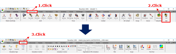
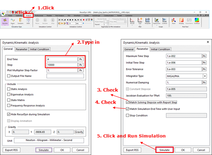
In the Analysis tab, click the Dyn/Kin icon to open the Dynamic/Kinematic Analysis dialog box. Enter information in End Time and Step. In the Parameter tab of the Dynamic/Kinematic Analysis dialog box, select Match Solving Stepsize with Report Step and Match Simulation End Time with User Input. Then, click Simulate.
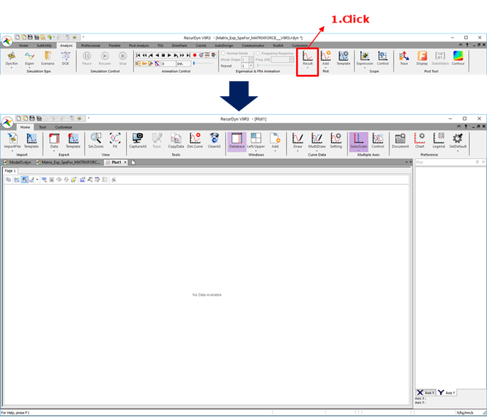
Click the Plot icon to open the Plot window, and then ensure that the results appear.