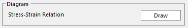
The Draw button, as shown in Figure 1, in the plastic material dialog box opens the Plastic Hardening Rule plot dialog box containing a plot of the stress-strain relationship defined by the current plastic material input data, as shown in Figure 2.
Figure 1 The Draw button in the Plastic Material dialog box
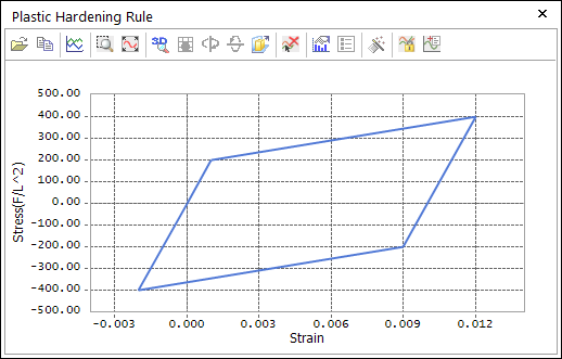
Figure 2 The Plastic Hardening Rule plot dialog box
The Plastic Hardening Rule dialog box contains a plot that corresponds to the axial stress versus the total axial strain that would be experienced by a specimen of material subjected to a tension and then a compression load in a uniaxial test. The load magnitude follows a pattern like the one shown in Figure 2.

Figure 3 Hypothetical axial load applied to a specimen
For the bilinear and nonlinear isotropic hardening (with or
without the kinematic hardening), the load  is 2x the initial yield stress. In
the case of the nonlinear isotropic hardening, though, it is possible that the
is 2x the initial yield stress. In
the case of the nonlinear isotropic hardening, though, it is possible that the
 is unreachable. This
occurs when
is unreachable. This
occurs when  ,
,  , and
, and  . Therefore, in the case that and , the load
  that is used is
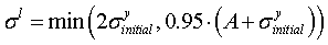
In the case of the multi-linear isotropic hardening, the load
is chosen so that at time  , the yield stress is
  . Note that if the kinematic
hardening is used,
. Note that if the kinematic
hardening is used,  because the kinematic hardening
introduces a back stress
because the kinematic hardening
introduces a back stress  .
.
The slope of the total axial strain to axial stress curve during the plastic flow is expected to be

where  is the sum of the
isotropic hardening modulus and the kinematic hardening modulus.
is the sum of the
isotropic hardening modulus and the kinematic hardening modulus.
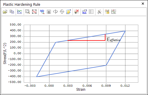
Figure 4 The slope of the total strain vs. stress
References
Simo, J. C., and Hughes, T. J. R., Computational Inelasticity, Springer, 1998