 (a)
(a)
Many real engineering design situations such as rotating shafts, connecting links, automotive and aircraft components and many other cases, require multi-axial fatigue equations. The multi-axial effects complicate the analysis required for the prediction of fatigue behavior.
Biaxial fatigue algorithms are commonly used to take into account the multiaxial loading conditions. There are two common approaches used for bi-axial fatigue evaluations.
•The bi-axiality ratio method: it calculates fatigue results quickly. However, it becomes too conservative when the loading between two axes is not proportional.
•The critical plane method: it takes a lot of time in searching the critical plane but it’s more accurate than the other method.
Axiality Ratio Method
In this method, a proportional loading assumption is assumed so that it can count the stress or strain cycles in one direction and can decide the corresponding ones in other directions. This assumption implies:
•The principal axes remain unchanged during the loading.
•The bi-axiality ratio between two principal stresses (or strains) range is a constant.
The procedure of the Bi-Axiality Ratio Approach is as follows:
1. Find two principal axes (primary and secondary loading directions).
2. Calculate biaxial ratio.
3. Perform the rainflow counting for the stress or strain history in the primary loading direction.
4. When the stress or strain amplitude and mean stress of each cycle is obtained, the stress biaxial ratio is used to update the life equations.
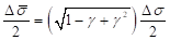
For the stress-based criteria, the effective stress amplitude is written as
(a)
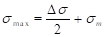
And the effective mean stress is
 (b)
(b)
Therefore, the user can get the life equation for stress-based criteria by using equations (a) and (b) with uni-axial life equations.
For the strain-based criteria, the user can get following life equations.
•Manson-Coffin
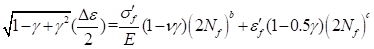
•Morrow
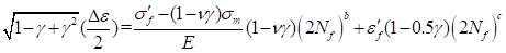
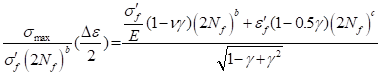
•Smith-Watson-Topper (S-W-T)
where
 ∶ Normal strain amplitude for a
cycle
∶ Normal strain amplitude for a
cycle
 ∶ Fatigue strength
coefficient
∶ Fatigue strength
coefficient
 ∶ Reversals to failure
 ∶ Fatigue strength exponent
(material property)
∶ Fatigue strength exponent
(material property)
 ∶ Fatigue ductility exponent
(material property)
∶ Fatigue ductility exponent
(material property)
 ∶ Fatigue ductility
coefficient
∶ Fatigue ductility
coefficient
 ∶ Fatigue strength
coefficient
∶ Fatigue strength
coefficient
 ∶ Mean stress for a cycle
 ∶ Elastic modulus (Young’s
Modulus)
∶ Elastic modulus (Young’s
Modulus)
 ∶ Poisson’s ratio
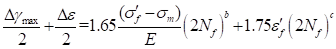
Critical Plane Method (Brown-Miller)
The Brown-Miller algorithm is the preferred algorithm for the most conventional metals to take into account the non-proportional biaxial loading. The following equations show the Brown-Miller life algorithm.
where
 ∶ Shear strain amplitude in the
maximum shear plane for a cycle
∶ Shear strain amplitude in the
maximum shear plane for a cycle
∶ Normal strain amplitude for a
cycle
∶ Fatigue strength
coefficient
 ∶ Mean stress for a cycle
∶ Elastic modulus (Young’s
Modulus)
∶ Reversals to failure
∶ Fatigue strength exponent
(material property)
∶ Fatigue ductility exponent
(material property)
∶ Fatigue ductility
coefficient