CMR of RS Theory

The connection degrees-of-freedom (DOF) for the flex body are equivalent to the exterior DOF of a superelement. In Nastran set terminology, this means the connection DOF are in the t-set. The interior DOF of the flex body component are part of the o-set. The union of the t-set and o-set is the f-set.

The first solution step of the CMR or RS method is to compute normal modes and static constraint modes. The normal modes are computed with the specified t-set DOF restrained. The normal mode shape matrix,  , can be used to transform the physical displacement uf (and its partitions ut and uo) into the generalized modal DOF, q. The transformation relation is

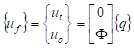                             (1)

The static constraint modes are static deflection shapes computed by applying unit deflections at the t-set DOFs. This is the same thing as performing a Guyan reduction on the o-set DOF. The static constraint modes transform full physical displacement uf into just the physical DOF, ut. The transformation relation is

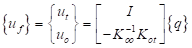                        (2)

The matrices Koo and Kot are partitions of the Kff stiffness matrix.

The normal mode transformation is a good reduction for the global dynamics and the constraint mode transformation is a good reduction for the local stiffness at the connection DOF. These transformations can be combined into a single transformation as

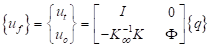                   (3)

The combined transformation captures both the global dynamics and the local stiffness of the component in the reduction.

In the second solution step, the transformation in equation (3) is used to mathematically reduce the model from the full physical DOF set to a reduced set of generalized modal DOFs and the t-set physical DOFs. The reduced DOF set size is equal to the sum of the number of normal modes and number of connection DOFs. Since the normal modes and static modes are not orthogonal to each other, the reduced mass and stiffness matrices are not diagonal as they would be with a pure normal mode reduction. However, a second modal solution is performed on the reduced system resulting in a new set of modes.

The final modes are orthogonal to each other and importantly, capture both global dynamics and local stiffness characterizations of the flex body. It is this second set of modes shapes that are exported to the flex body file. It should be noted that it is critical that all the modes of the reduced system should be solved in the second modal solution so that full global and local effects embodied in the reduction are retained.